
Safety Stock
Definition
Safety stock is an additional quantity of stock maintained to avoid stock-outs in the event of unforeseen events, such as higher-than-expected demand or delayed deliveries from suppliers.
Reminder : relationship between economic order quantity (EOQ) and safety stock (SS):
EOQ (Economic Order Quantity): This is the optimum quantity to order in order to minimize storage and ordering costs.
Safety Stock: This is a buffer stock that compensates for uncertainties in demand and supply.
Impact of QEC on safety stock:
If QEC is high : Large quantities are ordered at a time, reducing the frequency of orders. The average stock is therefore higher, reducing the need for a large safety stock.
If QEC is low : Orders are placed more often, increasing the risk of stock-outs between orders. In this case, a larger safety stock is needed to compensate for these risks.
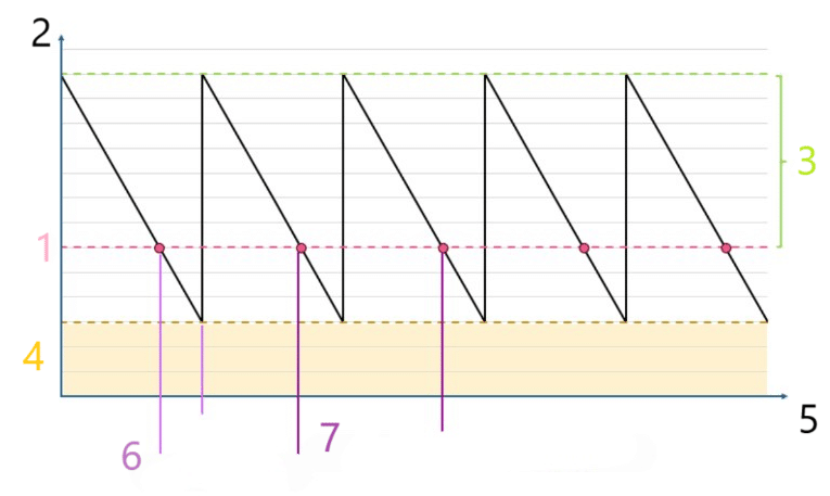
1 Reorder point
2 Stock
3 EOQ
4 Safety Stock
5 Time
6 Lead time
7 Replenishment lead time
Its main objectives are to :

1) Guarantee product availability despite fluctuations in demand
Customer demand can vary due to seasonal trends, promotions, or unforeseen events.
2) Absorb deviations in replenishment lead times
Immediate product availability improves the customer experience and reduces the risk of lost sales.
A good level of safety stock helps maintain a high service rate, reinforcing customer loyalty and the company’s image.
Suppliers can sometimes fall behind schedule due to logistical, production or transportation problems.
3) Improve service levels and customer satisfaction
Immediate product availability improves the customer experience and reduces the risk of lost sales.
A good level of safety stock helps maintain a high service rate, reinforcing customer loyalty and the company’s image.
Reorder Point = Safety Stock + (Average Sales × Average Lead Time)
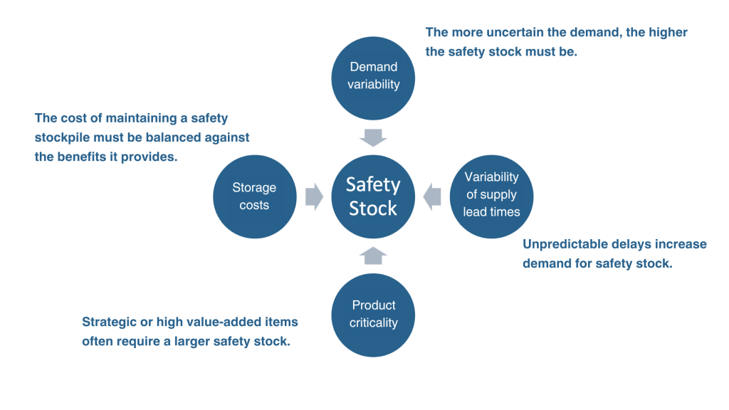
Several factors can influence safety stock:
Simplified formulas
In cases where demand fluctuates little, we use the formula :
Link between safety stock and ROP :
Note: The SS does not modify the QEC, but acts as a complement to absorb uncertainties.
For moderate fluctuations, SS can be calculated by taking into account the operational risk associated with significant fluctuations (in sales and lead times):
SS = Maximum Sales × Maximum Lead Time − Average Sales × Average Lead Time
Worst-case scenario for the company: demand is at its maximum, but restocking takes a long time.
Standard situation: demand and lead times follow typical values observed in historical data.
The difference between these two terms (maximum – average) reflects the level of protection needed against uncertainties. In other words, the greater the difference, the greater the risk of fluctuation, and therefore the greater the safety stock required.
Example:
Let be the number of sales and the lead times for the supply of an item in the year 2024. Calculate its safety stock.
| Jan | Feb | Mar | Apr | May | June | July | Aug | Sept | Oct | Nov | Dec | |
| Sales (unit/day) | 80 | 115 | 56 | 78 | 127 | 43 | 158 | 86 | 81 | 105 | 94 | 118 |
| Delay (days) | 2 | 4 | 10 | 6 | 3 | 2 | 5 | 3 | 7 | 12 | 4 | 7 |
Correction :
According to the table above:
Maximum sales: 158 units/day
Maximum lead time: 12 days
Average sales: 95 units/day
Average lead time: 5 days
So,
SS = 158 × 12 – 95 × 5 = 1896 – 475 = 1421 unités
If we use only the average sale and the average lead time, we anticipate only 475 units to cover demand;
In the event of an extreme situation, we would need 1,896 units;
The risk here is the difference between what is stocked on average (475 units) and what is needed in a pessimistic scenario (1896 units), i.e. 1421 units.
Normal law
When demand fluctuates: taking account of demand uncertainty
SS = Z × σV × √(Average Supply Lead Time)
With Z the security coefficient and σV the standard deviation of sales
When lead times fluctuate: taking into account uncertainty about lead times
With Z a safety coefficient and σV the standard deviation of sales
When lead times fluctuate : taking account of uncertain timescales
With Z a safety coefficient, V̅ the average sales and σD the standard deviation of lead times
Demand and lead times vary but do not influence each other:
Here, Z is the safety factor based on the desired service level.
σV is the standard deviation of demand.
σD is the standard deviation of lead time.
V̅ is the average demand.
This formula assumes that demand variability and lead time variability are independent.
Demand and lead times vary but influence each other:
This model incorporates a correlation between variations in demand and variations in replenishment lead times.
It is more accurate when these two factors influence each other.
Limits of the Normal Law Approach
Target service rate ≠ actual service rate
The method optimizes the frequency of stock-outs during a replenishment cycle.
Companies, on the other hand, often measure the total percentage of stock-outs over a wider period, which can distort the assessment of the required safety stock.
Poor performance for low sales volumes
When sales are low, fluctuations may appear proportionally greater, making normal distribution models less reliable.
Does not take seasonality into account
Seasonal variations (periods of high or low demand) are not taken into account, which can lead to errors in safety stock calculations.
Underestimation of extreme cases
Demand and lead times do not always follow a symmetrical distribution.
Sharp falls in sales and late deliveries are frequent, but the opposite (extremely high sales and very early deliveries) is rarer.
The normal model may therefore underestimate the risk of stock-outs in extreme situations.
Example :
Let’s go back to the previous example. Calculate the safety stock for a safety factor of 1.65 (the data are assumed to be independent).
| Jan | Feb | Mar | Apr | May | Jun | Jul | Aug | Sept | Oct | Nov | Dec | |
| Sales (units / day) | 80 | 115 | 56 | 78 | 127 | 43 | 158 | 86 | 81 | 105 | 94 | 118 |
| Delays (days) | 2 | 4 | 10 | 6 | 3 | 2 | 5 | 3 | 7 | 12 | 4 | 7 |
Correction:
According to the table above:
Standard deviation of demand: 32 units/days
Standard deviation of lead time: 4 days
Average demand: 95 units/day
Average lead time: 5 days
This gives :
Example
Calculate the Safety Stock of each ABC class of Units using the following three methods:
Mean-max method
Normal law with uncertainty on demand
Normal law with uncertainty on demand and independent lead time
Note:
For a service rate of 85%, Z= 1.04 (normal law table).
Lead times correspond to “Purchase Leadtime” or “Manufacturer Leadtime”.
Demand corresponds to sales.
Calculate the Safety Stock for each ABC class of Units using the following three methods:
- SS = (Delay Max × Sale Max) – (Delay Centile80 × Sale Centile80)
- SS = (Delay Centile95 × Sale Centile95)- (Delay Centile80 × Sale Centile80)
- SS = (Delay Centile80 × Sale Centile80)- (Delay Centile50 × Sale Centile50)
Note:
We no longer use the service rate but the percentiles
Demand corresponds to “max sale” and “min sale”.
Summary
Demand and lead times vary little:
Taking operational risk into account
Order point
Demand fluctuations
Fluctuation in lead times
Lead times and demand fluctuate, but do not influence each other
Delays and demand vary and influence each other
Manufacturing and production orders
Definition
Production Order (PO) : Definition and contents
A Production Order (PO) is an essential document in production management. It authorizes and supervises the manufacture of a product in a defined quantity and for a precise deadline.
Role of the PO
It guides the transformation of raw materials into finished products.
It centralizes all the information needed to ensure that production runs smoothly and conforms to requirements.
Information contained in an OF
1. Identification
- Unique order number.
- Issue date.
- Person responsible for the order (workshop manager, planner, etc.)
2. Product : product designation or specific reference.
3. Quantity : number of units to be produced.
4. Deadlines : estimated start and end dates for production.
5. Bill of materials : list of raw materials and components required (routing, detailed sequence of manufacturing operations (assembly, machining, quality control, etc.).
Definition: Derived from the OF, a Production Order specifies the specific tasks to be carried out on a machine, production line or workstation.
| Aspect | Work Order (WO) | Production Order (PO) |
| Level | Global (product or series) | Detailed specific operations |
| Objective | Overall planning and launch | Execution of specific steps |
| Example of information | Production, quantities, deadlines | Workstation, machine, duration |
Objectives and uses of OF/OP
Efficient planning: Define raw material, equipment and labor requirements to ensure an optimized production flow.
Traceability: Track each manufacturing step to guarantee quality and comply with production standards.
Cost control: Compare estimated and actual costs to optimize profitability and avoid financial discrepancies.
Continuous improvement: Identify bottlenecks and inefficiencies to optimize processes and increase productivity.
OF/OP challenge
From OF to OP :
- OF creation :
An OF is generated in response to a customer request or a production plan.
Example: Production of 500 units of a product. - Definition of POs:
The OF is broken down into OPs to allocate tasks.
Example: Cutting, assembly and finishing operations. - Execution and follow-up:
OPs are carried out in the field, with real-time tracking thanks to tools such as badging. - Closing the OP:
Once all OPs have been completed, the OF is closed, and the products are stored or delivered.
Case study
A company receives an order for 1,000 wooden chairs to be delivered in 15 days. Each chair requires :
- A cutting operation (2 minutes per chair).
- An assembly operation (3 minutes per chair).
- A finishing operation (1 minute per chair).
Correction:
1. Creation of an OF for the global order (1,000 chairs).
2. Definition of OPs:
– Cutting: 1,000 chairs x 2 minutes = 2,000 minutes.
– Assembly: 1,000 chairs x 3 minutes = 3,000 minutes.
– Finishing: 1,000 chairs x 1 minute = 1,000 minutes.
3. Resource planning (machines, personnel).
4. Production tracking via badge system.
A company manufactures wooden tables. Each table goes through three production stages:
Wood cutting ;
Assembly;
Finishing (sanding and varnishing).
Data :
The customer order is for 100 tables.
Time required per stage (for one table):
Cutting: 5 minutes
Assembly: 10 minutes
Finishing: 8 minutes
Each step requires a specific machine or operator.
Questions :
Create an OF to respond to this order. Describe the general information it must contain (quantity, lead times, etc.).
Break this OF down into POs for each stage. Indicate the specific tasks and associated times.
If a machine breaks down during finishing and is only running at 50% capacity, how much extra time will be needed to finish production?
Suggest a solution to reduce production times by optimizing OPs.
Correction:
- OF :
- Product: Wooden table
- Quantity to be produced: 100 units
- Estimated overall lead time: Calculate the total time required for all stages in series.
- Stock required: Check that raw materials are available.
- Priority: Normal/urgent (depending on customer requirements).
2. OP :
- OP1: Wood cutting
Total time: 100 × 5 = 500 minutes
Resource: Cutting machine - OP2 : Assembly
Total time: 100 × 10 = 1000 minutes
Resource: Assembly station - OP3 : Finishing
Total time: 100 × 8 = 800 minutes
Resource: Finishing station (sanding and varnishing)
3. Impact of failure :
- Machine running at 50% of finishing capacity
- Overtime: 800/0.5= 1600 minutes
- Additional time: 1600 – 800 = 800 additional minutes
4. Optimization :
- Introduce a second machine for finishing.
- Reorganize tasks in parallel (assembly and finishing on separate batches).
- Check whether finishing can be subcontracted.
Badging time
Definition
Definition of badge time
Badging time is the time recorded when an operator, machine or workstation starts and finishes a specific task. This time is captured using a badging or electronic recording system, enabling each operation to be traced precisely.
The benefits of badge time
Badging time is essential for several reasons:
– Measuring the actual duration of operations: This lets you know exactly how long a task has taken.
– Analyze operator and machine productivity: You can assess whether or not operators or machines are efficient during production.
– Calculate production costs accurately: The actual time spent on each task can be used to determine actual production costs.
– Identify discrepancies between standard scheduled time and actual time required: This helps identify anomalies or inefficiencies in the production process.
– Trace activities for quality control or human resources management purposes: Time badging enables operations to be tracked and managed, guaranteeing good quality and human resources management.
| Badging time | Meaning |
| Human operators | Time spent on each task |
| Machines | Operating, downtime or maintenance time |
| Specific tasks | Time associated with a specific step in the manufacturing process |
| Controls | Follow-up of OFs or OPs on the production line |
Related calculations
Total Badging Time :
Operator Productivity :
Gap Analysis :
Advantages and limitations
Digital tools used for badging :
ERP (Enterprise Resource Planning) systems: These systems track all company processes, including production, human resources and inventory management. They enable integrated, company-wide monitoring of operations.
MES (Manufacturing Execution Systems): These systems are specifically designed to manage production tasks. They track the progress of production orders and operations carried out on machines and workstations in real time.
RFID or biometric badges: These technologies automatically capture the start and end of operations without manual intervention, for example by scanning an RFID badge or using biometric recognition (fingerprints, facial recognition, etc.).
Advantages of badging :
Accuracy: Badging enables precise measurement of the actual time spent on each operation, thus avoiding approximations.
Traceability: It provides detailed, comprehensive tracking of human activities and machine actions, which is useful for production and quality management.
Optimization: Badging helps to identify inefficiencies, bottlenecks or delays in the production process, thus optimizing resource management and reducing costs.
Limitations :
Cost: Implementing badging systems, such as ERP systems, MES, or RFID and biometric badges, can represent a substantial investment in terms of hardware and software.
Reliability: There is a risk of human error, for example, if an operator forgets to badge at the beginning or end of a task. This can distort the data collected.
Human impact: Badging can be perceived as a means of excessive control, which can undermine employee motivation or create tensions, especially if employees feel intrusively monitored.
Case Study
A production line assembles smartphones. Each operator badges in
and end of job. Here’s a table summarizing their data:
| Operator | Task | Standard time (min) | Badging time (min) |
| Alice | Screen mounting | 20 | 22 |
| Bob | Battery installation | 15 | 14 |
| Clara | Quality control | 10 | 12 |
Calculate the total badge time, the expected standard time and the overall deviation. Did any of them exceed the scheduled time?
Correction :
Total badge time : 22 + 14 + 12 + 48 min
Expected standard time : 20 + 15 + 10 = 45 min
Overall deviation : 48 – 45 = 3 min
Here is a quiz to practice these different concepts: 🌐 QCM Link