
The revenue
General formula
To characterize a company’s financial flows, sales are a common and indispensable performance indicator. It can be calculated over different periods (annual, quarterly, monthly, etc.) and is expressed as:
Sales = Sales prices × Quantity sold
Note: To better understand the impact of different parameters on the company, sales can be classified by specific features (sales by family, by compliant items, by program, etc.).
Link with the supply chain
In the supply chain, sales data is used to:
- Prioritize efforts: Identify the most profitable customers, products, families, and programs. Analyzing the sales distribution helps pinpoint items generating the most revenue.
- Detect inefficiencies: Identify items without orders, pricing anomalies, dormant stock, and products covered by special commercial policies (e.g., free samples).
- Forecast and plan: Anticipate future needs based on trends and projections by extrapolating data and applying a growth rate.
Multidimensional Sales Analysis
Temporal criterion: months and years
→ Analyzing revenue by period helps identify seasonal or annual trends.
Key questions to ask:
What is the total revenue generated in a given year?
Are there months when sales are particularly high or low?
Is there a growth or decline trend over multiple years?
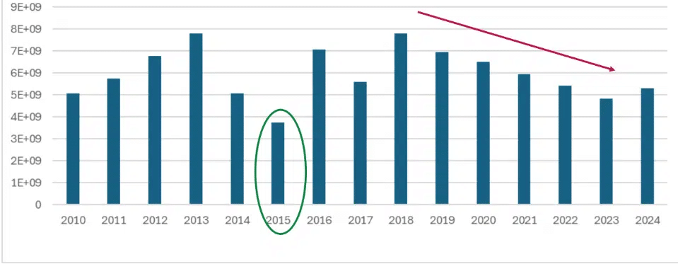
Graph showing the evolution of the total annual revenue over the years
o Decline in revenue over the last 6 years → Identification of a trend
o The least profitable year → Identification of the reasons impacting this revenue decline
Categorical criterion: product family
→ Analyzing revenue by family helps to identify which product groups generate the most revenue.
Key questions to ask:
Are there any low-profit or slow-moving families?
Which product family is the most successful?
What is the share of each family in the total revenue?
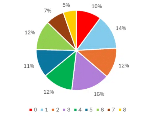
Graph showing the percentage by family of the revenue of 2024
o Family 3: the best performing family of 2024
o Family 8: the least profitable family of 2024
Crossing criteria
→ Crossing multiple criteria allows for a more detailed analysis.
Key questions to ask:
Which product family had the best sales during a specific year?
Are there any product families whose sales increase or decrease significantly over time?
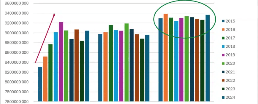
Graph showing the annual revenue evolution for each family
o Family 0: experienced strong growth for 5 years before stabilizing → increased marketing efforts and stock
o Family 2: the highest revenue-generating product each year → flagship product with high turnover rate
Key indicators
The service rate
Definition: The service rate measures the efficiency of a company’s production chain. It also reflects the company’s ability to meet customer demands effectively.
Service Rate = Number of orders delivered on time / Number of orders
| Part Number | Quantity | Order | Delivery |
| 1112326193 | 73 | 27/10/2022 | 27/10/2022 |
| 1112326193 | 39 | 30/10/2022 | 30/10/2022 |
| 1112326193 | 12 | 01/11/2022 | 05/11/2022 |
| 1112326193 | 66 | 03/11/2022 | 09/11/2022 |
| 1112326193 | 36 | 05/11/2022 | 05/11/2022 |
| 1112326193 | 59 | 10/11/2022 | 09/11/2022 |
| 1112326193 | 62 | 14/11/2022 | 17/11/2022 |
| 1112326193 | 24 | 14/11/2022 | 13/11/2022 |
| 1112326193 | 54 | 16/11/2022 | 16/11/2022 |
| 1112326193 | 8 | 19/11/2022 | 22/11/2022 |
| 1112326193 | 64 | 23/11/2022 | 23/11/2022 |
| 1112326193 | 63 | 24/11/2022 | 24/11/2022 |
| 1112326193 | 58 | 28/11/2022 | 26/11/2022 |
| 1112326193 | 1 | 01/12/2022 | 01/12/2022 |
Example:
Let’s calculate the service rate for the following sample: Only 4 orders were not delivered on time (they are marked in red).
Service Rate = 10 / 14
⟹ Service Rate = 71.43%
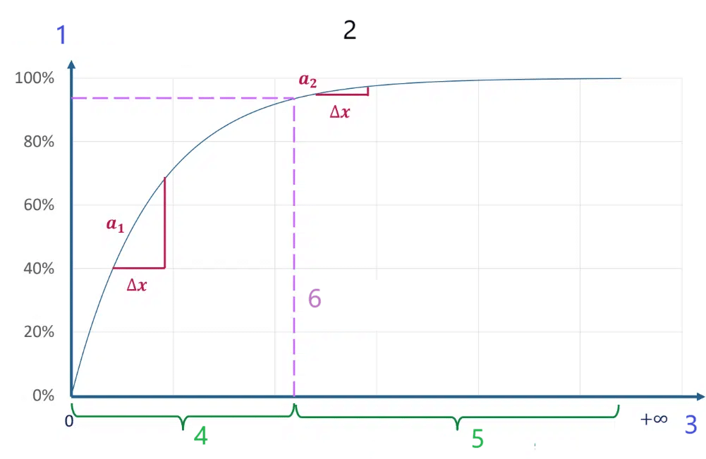
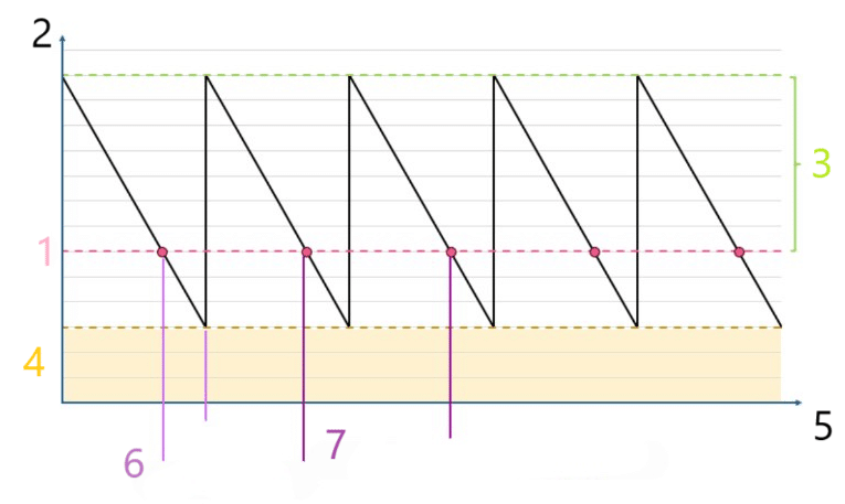
For the same stock variation ∆x, the variation in the service rate can be very different.
Law of diminishing returns:
• An insufficient stock reduces the service rate.
• An excessive stock does not always significantly increase the service rate.
1 Service rate
2 Evolution of the service rate according to stock levels
3 Stock level
4 Understocking area
5 Overstocking area
6 Optimal level: balance
Taking into account the quality parameter:
In addition to delivery times, it may be interesting to consider the quality of service:
How many orders were delivered on time and in good condition?
τQ = (Orders delivered on time − Disputed orders)/Total number of orders
Weighted service rate:
To understand the actual impact of the company’s work, the weighted service rate is used:
τQ = (Orders to be delivered − Late orders)/Total number of orders received
How to optimize the service rate?
• Use of an ERP (Enterprise Resource Planning)
Software used by companies to manage their daily activities such as accounting, purchasing, project management, risk management and compliance, as well as Supply Chain operations.
• Cost analysis
Identify the costs related to inventory, orders, and stockouts in order to prioritize actions.
• ABC Method
↳ See Chapter 3: THE ABC Method
Classifying products based on their importance also allows for prioritization.
• Optimal safety stock
A safety stock adapted to demand fluctuations and lead times helps prevent stockouts.
Order compliance rate
Definition: The order compliance rate is a key indicator used to measure a company’s ability to meet customer expectations when fulfilling orders.
Order Rate = Number of compliant orders / Total number of orders

- Inventory
- Service
- Human resources
- MRP
- Purchasing
- CRM
- Sales
- Financials
- Production
Note:
Compliance can take into account several criteria such as delivery times, quantities, product quality, associated documentation…
Example:
The table below lists the data for a particular product over a given period with a restocking lead time of 1 week.
The associated costs are as follows:
• Current safety stock: 50 units
• Average demand per order: 130 units
• Standard deviation of demand: 20 units
• Target service rate: 95%
• Safety factor associated with a 95% service rate: 1.645
1. Calculate the basic service rate.
2. Calculate the service rate for an optimal level using the safety stock formula:
SS = Z. σ. √LT where Z is the coefficient corresponding to the target service rate, σ is the standard deviation of demand, and LT is the lead time.
| Order | Requested quantity | Delivered quantity | Quantity in compliance | Deadlines met (Y/N) |
| 1 | 100 | 90 | 85 | Y |
| 2 | 200 | 200 | 190 | N |
| 3 | 150 | 130 | 130 | Y |
| 4 | 80 | 80 | 75 | Y |
| 5 | 120 | 100 | 95 | N |
Correction:
1. Basic service rate: τ = √3 / √5 = 60%
2. SS = Z. σ. √LT = 1.645 × 20 × √7 = 87 units
Factors impacting the conforming order rate
Factors impacting the conforming order rate
Compliance criteria
Benefits associated with this rate
Economic Order Quantity
EOQ
Economic Order Quantity (EOQ) is a fundamental concept in inventory management. It is used to determine the optimum quantity to order in order to minimize the total costs associated with inventory management, which generally include ordering costs, storage costs, and out-of-stock costs. It determines how many items to order and when to order them.
EOQ is based on several key factors:
• Unit ordering cost (Ccu): This is the cost associated with placing an order (administrative costs, transport, etc.).
• Unit storage cost (Csu): This corresponds to the costs associated with holding stock, such as storage space, insurance, inventory management, etc.
• Demand (D): The quantity of product demanded over a given period. Demand may be stable or variable, depending on the type of product.
EOQ is calculated using the following formula:QEC = √( (2 × D × Ccu) / Csu )
EOQ is intrinsically linked to the reorder point.
• EOQ determines how many items to order at each replenishment.
• The reorder point determines when to order based on stock levels.
1 Reorder point
2 Stock
3 EOQ
4 Safety Stock
5 Time
6 Lead time
7 Replenishment lead time
Thus, EOQ indirectly influences the reorder point, as an EOQ that is too large or too small can alter consumption during the lead time or the frequency of orders.
Once EOQ is set, it is used to calculate the stock level to maintain.
The reorder point is the stock level at which an order must be placed to avoid a stockout.
Reorder Point = Safety Stock + Demand during Lead Time
Example:
A company consumes 12,000 units of a product per year. The cost per order is €50, and the holding cost per unit is €2. The safety stock for this product is 400 units, and its lead time is 5 days. We assume a constant daily consumption.
1. Calculate the EOQ.
2. Calculate the reorder point.
3. Conclude.
Correction:
1. EOQ:
EOQ = √( (2 × 12000 × 50) / 2 ) = 774.6 units
2. Since daily consumption is constant, we have:
Cj = D / 365 = 12000 / 365 = 32.9 units per day.
Thus: ROP = 5 × 32.9 + 400 = 564.4 units.
3. Conclusion:
As soon as the stock drops to 565 units, an order of 775 units is placed to minimize costs.
Cost management
The EOQ is also the quantity of items to order for which the total cost is minimized.
To determine the minimum total cost associated with this EOQ, we can use the following formulas:
• The holding cost for a quantity equal to the EOQ:
Cs = Csu × (EOQ / 2)
• The ordering cost at the EOQ:
Cc = Ccu × (D / EOQ)
• The minimum total cost:
C = Cc + Csu
Example:
A company manages three items A, B, and C with the following data:
| Annual demand | Unit ordering cost | Unit holding cost | |
| Item A | 15000 units | 30€ | 2€ |
| Item B | 8000 units | 50€ | 3€ |
| Item C | 20000 units | 40€ | 1.5€ |
1. Calculate the EOQ for each item.
2. Compare the total costs for the three items based on the calculated EOQ.
3. After review, it is observed that the annual demand for item A ranges between 14,000 and 16,000 units. Calculate an EOQ range based on the extremes of the demand and discuss the importance of forecasting demand to adjust orders.
Correction:
1. EOQ for each item:
Item A: EOQA = 671 units
Item B: EOQB = 517 units
Item C: EOQC = 1033 units
2. Total costs for each item:
Item A: C = 30 × (15000 / 671) + 2 × (671 / 2) = 1342€
Item B: C = 50 × (8000 / 517) + 3 × (517 / 2) = 800€
Item C: C = 40 × (20000 / 1033) + 1.5 × (1033 / 2) = 1550€
3. After review: EOQA ∈ [648 ; 693] units.
An inaccurate demand estimate leads to poor order planning (frequency and quantities).
This can cause:
• Stockouts (in case of underestimating demand);
• Unnecessary overstock (in case of overestimating demand).
Graphical study
It is possible to determine the EOQ graphically. To do this, we plot the holding costs and ordering costs as a function of the order quantity.
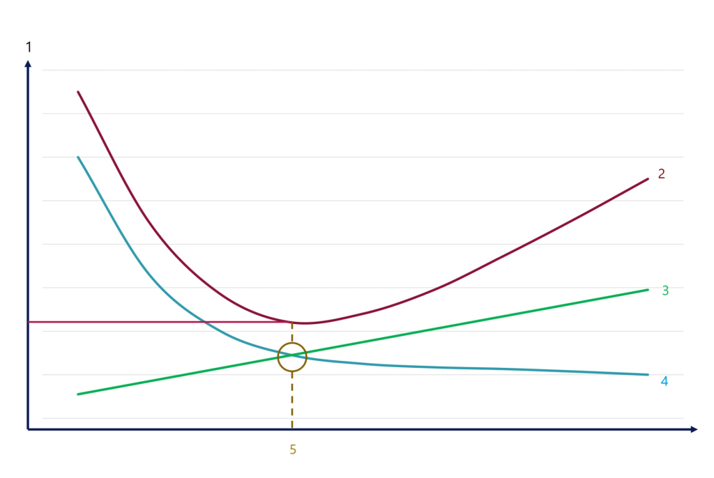
1 Cost
2 Global Cost
3 Storage Cost
4 Storage Cost
5 EOQ Cost
Minimum of total costs at the EOQ level
Increase in holding costs as the order quantity increases: → Maintaining a higher inventory to cover demand.
Decrease in ordering costs as the order quantity increases: → Reduction in the number of orders required.
Exemple : An item has an annual demand of D = 112 units. The unit ordering cost is Ccu = 14, and the unit holding cost is Csu = 4.
- Calculate the EOQ.
- Verify its value graphically.
- Determine the total costs associated with the EOQ.
- Compare these costs with those obtained if the company orders 49 units per order.
Correction :
1. EOQ = √((2 × Demand × Ccu) / Csu)
= √((2 × 112 × 14) / 4)
= 28 units
2. To verify graphically, we plot:
• Ordering cost:
Cc = Ccu × (D / Order Quantity)
= 14 × (112 / Order Quantity)
• Holding cost:
Cs = Csu × (Order Quantity / 2)
= 4 × (Order Quantity / 2)
The EOQ corresponds to the quantity that minimizes the total cost C = Cs + Cc, meaning the EOQ is the order quantity where Cc = Cs.
3.The ordering cost associated with the EOQ is:
Cc = 14 × (112 / 28) = 56€ The holding cost associated with the EOQ is:
Cs = 4 × (28 / 2) = 56€ (we verify that Cc = Cs) The minimum total cost is therefore: C = 112€.
4.Now, we calculate the costs for an order quantity of 49 units. The ordering cost for this quantity is:
Cc = 14 × (112 / 49) = 32€ The holding cost for this quantity is:
Cs = 4 × (49 / 2) = 98€ The total cost is therefore: C = 130€. By ordering 49 units instead of 28, the company ends up paying more.
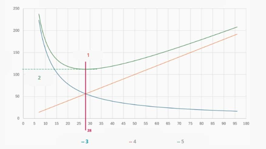
1 : EOQ
2 : Minimum overall cost
3 : Order cost
4 : Stock cost
5 : Overall cost
Exercise
To conclude, here is an exercise to practice with a database. The questions are as follows:
Sales Calculation
1. In the “Data” tab, calculate the revenue for each item (an item corresponds to a part number).
2. Create a Pivot Table (TCD) by month and generate a chart.
3. Create a Pivot Table by year and family.
Rolling Annual Revenue
4. Calculate the company’s annual revenue.
– You can use the previously created Pivot Table to obtain:
5. Calculate the annual revenue per program for each year.
6. Identify the top customers by amount and quantity per customer.
Service Rate Based on Revenue
7. Calculate the service rate over a full year (as of today) = on-time delivered orders / total orders.
– Then, simply apply the formula.
8. Calculate the monthly service rates for 2022.
9. Calculate the monthly service rates for 2022 for Family 1.
Economic Order Quantity
10. Calculate the economic order quantity for each item.
– Here, “Annual Quantity” corresponds to demand.
– A Pivot Table is used again.
Compliance Rate
11. Calculate the perfect order rate over a full year (January 1st – December 31st) = Compliant Quantity / Delivered Quantity.
12. Calculate the order rate for 2023, by month.
13. Calculate the order rate by program.
📂 Excel file to download: Download here
✅ Correction: View correction
📥 Corrected Excel file: Download corrected file
Here is a quiz to practice these different concepts: 🌐 QCM Link